Linearity

What one normally learns in an introductory linear algebra class is that vectors are a group of numbers, such as:

It turns out that this is wrong, and this article will go in depth as to why that is. We will then use this new way of seeing vectors to revisit what a matrix really is.

That being said, I highly recommend watching 3Blue1Brown’s Essence of linear algebra. It’s great and the visualizations are impeccable. You will feel like your linear algebra class hasn’t taught you anything. Throughout this article, I will assume that you have watched the series. The goal of this article is actually to push that series even further.

Mathematics and Set theory crash course

Before we actually start defining what a vector space is, it’s useful to know a pattern used extensively in nearly all of mathematics. When a mathematician wants to create a new mathematical object (such as the real numbers, complex numbers, vector spaces, etc.), she starts by defining a set. This set will contain the different values that the mathematical object can take. She then defines operations (that we call structure) that will determine the available actions that one can take with respect to the mathematical object. For example, the set of real numbers defines two operations: addition and multiplication.

As you shall now see, this is exactly how vector spaces are built!

Vector spaces

What’s a vector space? Well, let’s start with the definition from Wikipedia and go from there.

A vector space over a field F is a set V together with two operations [addition and scalar multiplication] that satisfy [some eight axioms].

Visually, this is what a vector space looks like:

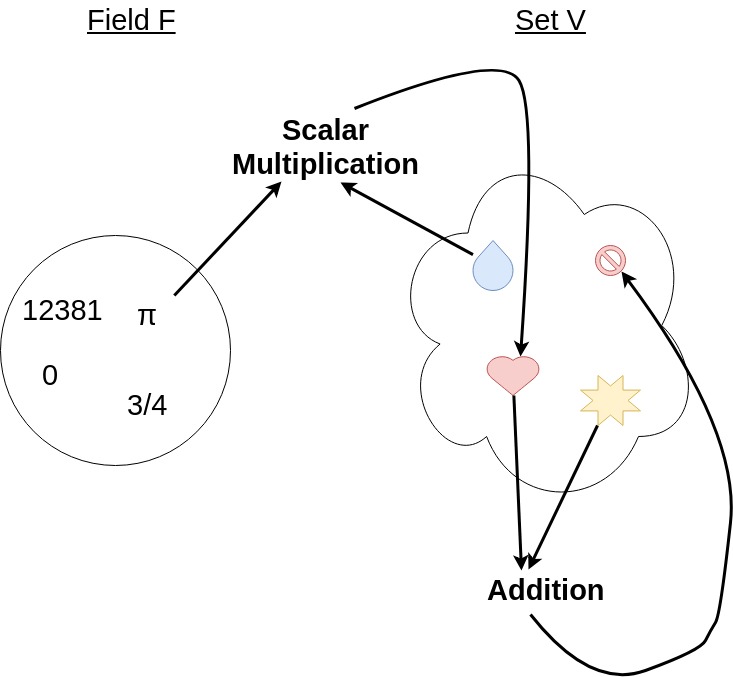
You can refer back to this image as we dissect the definition.

Field

To understand the vector space definition, we first need to understand what a field is. A field is a generalization of numbers. That is, the axioms (or “requirements”) that a set must follow in order to be considered a field makes it act just like the real numbers. Those rules are, for example, that there must be an addition operation and a multiplication operation (and your set is closed under both of them), both of these operations must be associative and commutative, that multiplication must distribute over addition, and so on. If you feel like this crash course isn’t satisfactory, I recommend watching the first two lectures of the real analysis course given by Francis Su on Youtube.

For the purposes of this article, every time you read field, you should think the set of real numbers. We will refer to the elements of the field as scalars.

Vector addition and scalar multiplication

We also need to understand what both of the operations referred to by the definition are. Let’s start with addition.

The addition operation is a function that associates two elements of our set V to a single element of V. Formally, we write V x V → V, where the x notation refers to the cartesian product. In case you’re not used to the concept, you can see the cartesian product as enumerates all the possible ordered pairs of the set, and the addition operation associates an element of V to each one of these pairs. This is well explained in the first video of the abovementioned real analysis course.

The second operation, scalar multiplication, is a function that associates with each pair of element from our field and element from our set V some element in our set V. Formally, we write F x V → V.

The 8 axioms

But there’s a catch. You can’t define these two operations however you like! You need to make sure that they follow the 8 axioms. We won’t go over all of them one by one, but for the purpose of the exercise, I recommend you bring back your notion of vector as “an arrow in a coordinate system” for a second and verify that this arrow system really is a vector space (by checking that it satisfies all 8 axioms). You could also try to define addition some other way (e.g. taking the maximum of both coordinates, such that [3 2] + [1 4] = [3 4]). Which axiom is violated if you try doing that? All in all, those 8 rules are the only things that matter for this arrow system to be considered a vector space; anything else you can freely change.

To drive the point home: complex numbers are not vectors, even though they are often represented by arrows in space! And that’s because they don’t define a scalar multiplication operation, and they define an extra vector multiplication operation!

The bottom line

So what’s a vector space then? It’s a set of things (that we call… drum roll… vectors!) that can be added together and multiplied by numbers. That’s it. At its core, that’s what a vector is: an element of a set. It is not limited to being an arrow or a pair (or triplet, etc.) of numbers. It’s a member of whichever set you feel like defining, as long as you properly define how to add the elements together and multiply them by elements of a field.

Building our own “pi creature” vector space

In order to show that a vector space can really be anything we want as long as it fulfills the abovementioned axioms, we’ll build our own and use it throughout the rest of the article! At some point during 3Blue1Brown’s video about vector spaces, a “crazy type of vector space” about pi creature is glossed over. We’ll take it from there.

The elements of our set V will be pi creatures of a certain height who are a certain distance away from home. More specifically, a positive height will grow upwards, while a negative height will grow downwards (i.e. the pi creature would appear as if walking on the ceiling). Similarly, a positive distance away from home will mean “on the house’s right-hand side”, while a negative one will mean “on the house’s left-hand side”.

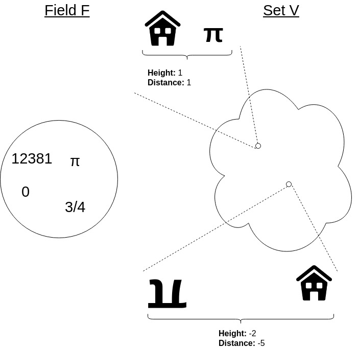
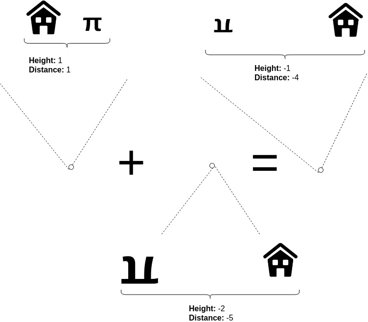
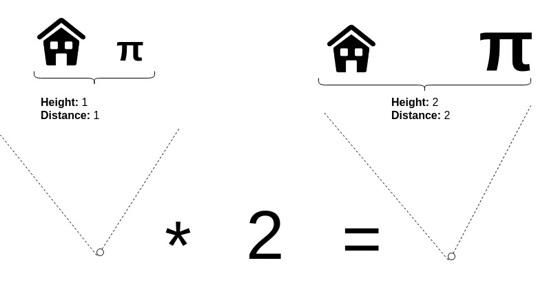
Addition between two pi creatures will be defined as adding the sizes and distances together, respectively. Scalar multiplication will be defined as multiplying both the size and the distance by the given number.

Addition

Scalar multiplication

Verifying that this is indeed a vector space is left as an exercise. Now that we have a toy vector space to play with, let’s move on.

Linear combination

In a linear combination of vectors, each vector is scaled (using the scalar multiplication operator) and then the scaled vectors are added together (using the addition operator). Mathematically, the linear combination l of vectors u, v and w is written

l = a * u + b * v + c * w , given scalars a, b, c and vectors u, v, w

Linear combinations are central to linear algebra, and why that is will become clear after we have introduced the concept of a basis.

The basis and dimensions

Another concept that you’ll hear over and over in linear algebra is the concept of a basis. Now, what is that and where does it fit in this whole “set V, field F, addition and scalar multiplication” way of thinking about vector spaces?

The basis

A basis is an arbitrarily chosen minimal set of vectors (called basis vectors) that can be linearly combined to form all of the vectors in our set. By “arbitrarily chosen”, we mean that there isn’t just one possible basis for a given space; actually, there are infinitely many of them! And by “minimal set”, we mean that the set is as small as it needs to be in order for all the vectors to be formed by a linear combination of the basis. A good way to test if your set is minimal is to try to linearly combine some of your basis vectors to reach another vector in your set of basis vectors. If you find a way to do that, then your set isn’t minimal.

Let’s take a second to discuss why we even care about defining basis vectors. The answer is pretty simple: computation. The basis allows us humans (or computers!) to perform computation on vector spaces. Since every vector in our vector space can be written as a linear combination of the basis vectors, we can say that the basis acts as a coordinate system on our vector space! And what do we get when we put a coordinate system on our vector space? We get vectors that look like coordinates! Like this:

And then introductory linear algebra classes can take a sweet shortcut and go right for the “this is what a vector is”. But it turns out that the distinction between the coordinates of a vector given a coordinate system (or basis) and the vector itself is crucial! Saying that [3 4] is the vector is the same as saying that your identity is [3 0] because you’re standing 3 meters in front of me (assuming that the first basis vector points in front of me of course).

Now that we’re comfortable with the concept of a basis, let’s move on to a concept that’s closely related: dimensions.

Dimensions

Everyone has an intuitive sense of what dimensions are: we live in a world that has 3 dimensions, a sheet of paper has 2 dimensions, and so on. But if you give me some funky vector space, how would I know how many dimensions it has? A vector space is just a set with some operations on top of it. What’s a dimension in this framework?

Basis vectors to the rescue! The number of dimensions is defined as being the number of vectors in any basis (all bases must have the same number of basis vectors, so pick your favorite basis). And when you think back to the 3 dimensional world and 2 dimensional piece of paper… This definition makes sense! Except now, you’re equipped with a robust definition that you can apply to any vector space thrown at you.

Basis for our pi creatures vector space

Let’s find a basis for our pi creatures vector space! We mentioned that basis vectors are arbitrarily chosen. Sweet! We’ll pick one at random, and see if we can scale it to reach all other pi creatures (since there’s only one pi creature for now, we don’t have any other vector to add it to, and so “linear combination” is reduced to “scalar multiplication”). If we aren’t able to reach all the pi creatures in our set, then we’ll randomly choose another vector to add to our set of basis vectors. Repeat.

Our first basis vector u will be the pi creature of size 5 and distance 3. Now if we scale this vector, we can reach vectors such as size 10 distance 6, size -50 distance -30, and so on. But we’ll never be able to reach size 5 distance 2 (amongst many others). Therefore this tells us that we need to add a new vector to our set of basis vectors.

Our second basis vector v will be the pi creature of size 5 and distance 2. With this second vector in our basis, we will be able to reach all other vectors through linear combination of the basis. This might not be immediately clear given these two vectors, but an easy way to verify this is to pick the basis size 1 distance 0, and size 0 distance 1. Then for any pi creature, you scale the first basis by the size of your pi creature, and you scale the second basis by you pi creature’s distance away from home. Since all basis have the same cardinality (or size), we can confidently claim that our u and v vectors form a valid basis.

Linear transformation

We’ve explored many concepts related to vector spaces themselves, and how to play around in them. However, many applications require a relation between two vector spaces to be defined. For example, if a vector represents the current position of an object in the world, you might want to define a function that will tell you where that object will be 1 second from now. Effectively, what you would be doing is mapping (or transforming) all of the points in the current vector space to where they would “land” in the vector space that represents these points 1 second in the future.

Now, in theory, you can define just about any transformation you’d want between the two spaces. However, we restrict ourselves to the linear ones (defined below). Let’s dive into why linearity is great.

What one learns in high school of linearity is that it looks like a line in space, and that the general equation for a line is f(x) = ax + b. This is a lie; such an equation is not linear. We rather say that it’s affine because of the + b. It turns out that this is a crucial distinction to make. In linear algebra, lines pass through the origin. This comes as a result of the two axioms of linearity:

L1: f(x + y) = f(x) + f(y)
L2: f(c * x) = c * f(x)

Let’s take a step back and think about why these two axioms capture what it means for something to be linear.

Intuitively, L1 says that a given input y causes the same change f(y) on the output irrespective where it “starts from”. In other words, y causes the change f(y) when it starts at 0 (i.e. f(0 + y)). L1 tells us that y causes f(y) even if it starts at x: f(x + y) = f(x) + f(y). The inputs pass independently through the function. As an analogy, imagine that you own a bubble gum machine where you have to twist the handle to get bubble gum out. If this machine is linear, then every tick will give you the same amount of bubble gum (e.g. 2 bubble gums). Tick once, get 2 bubble gums. Tick again (without resetting the handle), and get 2 more bubble gums. On the other hand, if the machine was nonlinear (e.g. exponential), then the first tick would give you 2 bubble gums. Then the second tick would give you 4, then 8, etc. Put into a mathematical language, x would be the number of ticks already registered on the handle when you get to the machine, and y would be the number of ticks you apply to the machine.

L2 says that scaling the input x by c will result in the same as mapping x to the output and scaling that resulting number by c. Using our bubble gum machine analogy, if the machine is linear, twisting 5 ticks is the same as 5 times what you get by twisting once. So given 2 bubble gums per tick, 5 ticks would give you 10 bubble gums, compared to 1 tick that gives you 2 (and 5 * 2 = 10).

For completeness, let’s also show mathematically that these two axioms hold for the equation of a line f(x) = m * x, though that doesn’t provide much intuition.

L1: f(x + y) = m * (x + y) = m * x + m * y = f(x) + f(y)

L2: f(c * x) = m * c * x = c * m * x = c * f(x)

Linearity for linear combinations

Note that L1 really works for an arbitrary number of variables summed together. For example, if you have f(x + y + z), then you can create a variable w = y + z and substitute it in the equation such that it becomes f(x + w) = f(x) + f(w). You can then substitute back f(w) = f(y + z) = f(y) + f(z). This trick can be applied recursively for an arbitrary amount of variables.

Now what if I told you that x = m * a for some constant m (and similarly for y = n*b and z = o*c)? We can substitute in to get

f(x + y + z) = f(m*a + n*b + o*c) = f(m*a) + f(n*b) + f(o*c) = m*f(a) + n*f(b) + o*f(c)

L1 and L2 naturally extend to any arbitrary linear combination!

Linear transformation recap

All in all, a linear transformation is a function that maps all vectors of a vector space to another vector space (potentially the same) such that L1 and L2 are satisfied.

Let’s now jump into our final subject: matrices!

The matrix

In light of all this new information, what’s a matrix? A matrix is a tool that allows us to compute linear transformations. In other words, we’ve already shown that a linear transformation is just a function. Therefore, it exists whether or not one can compute where each vector is mapped. However, when you want to actually use linear transformations… It’s awfully useful to know where vectors actually get mapped! A matrix tells you the computation to apply on the inputs in order to get the resulting output. This is similar to f(x) = x telling you the necessary computation to implement the identity function.

Now how exactly does the matrix do that? As a first principle, in order to compute on any mathematical object, you need a way to map this arbitrary mathematical object (e.g. a vector in a vector space) to numbers. This is exactly what a basis does! Recall that it effectively creates a coordinate system for all vectors in the vector space. In other words, matrices use the coordinates of vectors to perform computation.

Quick recap. A matrix helps you compute linear transformations using a basis as a coordinate system for vectors. And a linear transformation is a linear function from one vector space to another. It follows that the matrix assumes a basis in both the input and output vector spaces; and these bases need not be the same!

Fact #1: A matrix assumes a basis in both the input and output vector spaces of the linear transformation.

So how exactly does the matrix, a grid of numbers, do all of this? Let’s start by examining what happens when we send the first basis vector of our basis as input to the matrix. We’ll take a 2 dimensional vector for this example and will assume that the matrix is square.

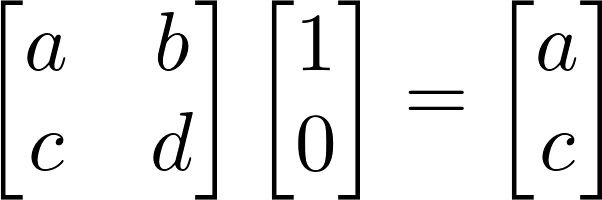
We get the first column of the matrix as output! And similarly for the second basis vector…

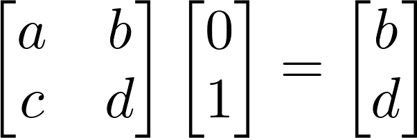
We get the second column! And so in other words, a matrix stores the coordinates of where the basis vectors get mapped by the linear transformation in its columns.

Fact #2: A matrix stores the coordinates of where the basis vectors get mapped by the linear transformation in its columns.

That’s it! We have all the pieces of the puzzle! We know where the basis vectors get mapped by the linear transformation, and the transformation is… linear! And therefore we know where all the vectors get mapped: the matrix maps the basis vectors to the output vector space, and then (using L1 and L2) it takes the linear combination of those to figure out where a given vector lands!

I now encourage you to go re-watch 3Blue1Brown’s videos on linear transformations and matrices, and on change of basis. Hopefully, you will see them in a new light!